Beyond VLOOKUP: Using Names & INDIRECT Function

Using named ranges has several benefits:

• Formulas are easier to follow if they use logical names instead of cell references.

• If your ranges change size, grow in length or some other dimension, you can easily change the definition of the range to accommodate the change. If you do not use names, you would have to change the cell references in all of your formulas.

• You can use the INDIRECT function to refer to ranges

Naming Cells/Ranges:
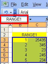
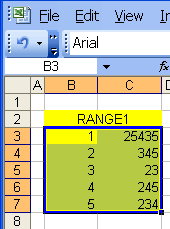
Highlight the cell or range of cells and then type the name in the cell reference box.














INDIRECT FUNCTION
This function is so powerful, so useful and so underutilized, I am afraid I might not be able to do it complete justice.

1. Indirect will allow you to reference individual cells by building a reference within a formula: Want to retrieve the value in Cell A1? Use this formula: =INDIRECT("A1")
   
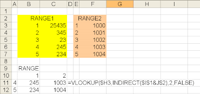
2. The true power of INDIRECT comes from its ability to build a name. Put the name of an variable or range in one cell and then add a number to it: Example Cell B9 contains RANGE and you want to reference RANGE2 =INDIRECT(B1,"2")
3. Building names is very handy when using functions like VLOOKUP that refer to ranges or arrays of data. See example below with two ranges of data: RANGE1 = B3:C7 & RANGE2 = E3:F7

Beyond VLOOKUP: OFFSET + MATCH = Insanity!

OK, so you are comfortable with VLOOKUP, but tired of counting columns to point the function to the data you are interested in. Wouldn't it be great to have the formula do the leg work and find the # of Columns or Rows to where your data lies?

I have the perfect formula for you, OFFSET. This formula allows you to set a reference cell and find data Relative to that cell.

We are using the same data set from the VLOOKUP example. Imagine we are tired of counting how many columns there are between Outlet and 1st Quarter Sales. We tell OFFSET to use Cell A6 as a reference. OFFSET will ask for the # of ROWS and COLUMNS to move from this reference cell.

Instead of simply counting the # of rows and columns, we embed the MATCH formula into OFFSET. MATCH is very simple and simply finds a cell the matches the data you input. In this example, we need to use the Outlet data to determine how many rows from the Reference cell to travel. Notice that the array we use with the MATCH function does not include any data. OFFSET only needs the number of ROWS we want it to move. The Outlet data is in Cells $A$7:$A$14. NOTE: Do NOT include your OFFSET Reference cell in the MATCH lookup_array. Use the number 0 for your match type. Using 0 will direct MATCH to find EXACTLY what you are looking for, just like FALSE in the VLOOKUP formula.

Repeat the above with another MATCH statement with the variable you are looking for, in this case, 1st Quarter Sales. This value must be EXACTLY as it is in your data array. I STRONGLY recommend copying this value from your data into your output sheet to assure you are looking for something MATCH will Identify. (Many raw data sets contain hidden spaces after the text).

I Would Like To Teach the World VLOOKUP!

If I could impart one piece of wisdom to members of the corporate rat race it would be: Use VLOOKUP! I see minions hunched over their keyboards cutting and pasting or WORSE, Inputting data by HAND! This is 2008 and we need to let technology do the work for us, not the other way around!

VLOOKUP is the simplest way to quickly grab data out of a large data set. Its uses are truly endless, but a typcial corporate exmaple would be the catch phrase, "REPORTING."

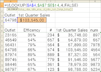
The Example to the left contains a list of Retail outlets identified by a 5 digit code typical of most raw data in a corporate environment.

How to Use Vlookup:

1. Lookup_Value: You want to return a specific value from a list of data. In this example, you must indicate which retail outlet you are concerned with. You hardcode 23165 in cell A3.

2. Table_Array: This is the raw data. The number (or text) you are searching for MUST be in the first column of this array. In our example, the Outlet is what we are searching for and it is in column A. CAREFUL if your list contains numbers, make sure they are not a number stored as text. You simply need to reformat the cells as numbers to overcome this issue.

3. Col_Index: VLOOKUP will VERTICALLY search the first column of your Table_Array to find the value you are searching for. Excel defines the first column as column 1. If you indicate 1 for the Col_Index, VLOOKUP will return the value you are searching for IF it is actually in the list you are searching. In this example, we want to find the 1st Quarter Sales which are in column 4.

4. [Range_Lookup] When in doubt, specify FALSE. I would go one step further and say ALWAYS use FALSE. This value tells VLOOKUP if you want to find an exact match in the Table_Array, or just something that approximates what you are searching for. If you use FALSE and the Table_Array does not contain the value you are searching for, VLOOKUP returns an Error. If you use TRUE and the value is not in the data, VLOOKUP may find a value similar to what you are looking for and return that corresponding value. In other words, there are few, if any times the average Excel user would want to use TRUE.